Orbitals Plotting#

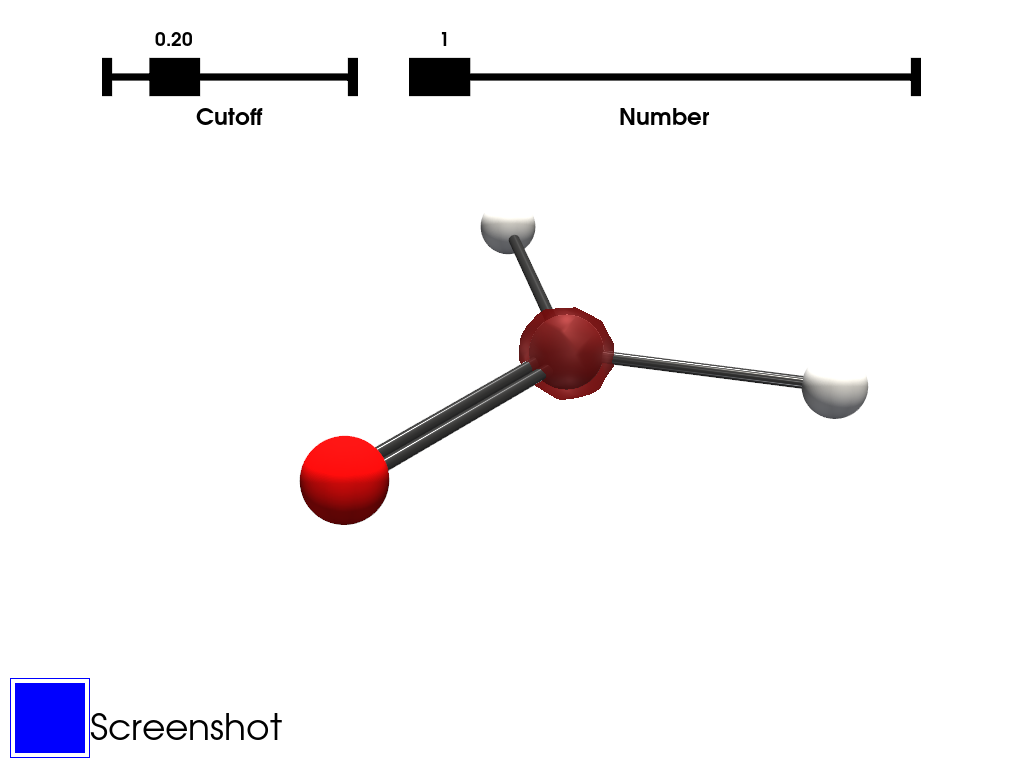
The orbitals can be plotted using two types of outputs :

  • Molden files recommended

  • Cube files

Molden files can be created from orca output by using the orca_2mkl tool.

Cube files can be created from orca output by using the orca_plot tool.

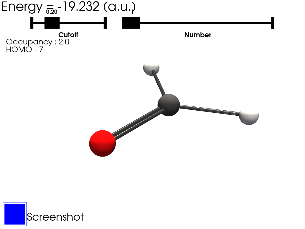
Using molden files instead of cube files allows to calculate the atomic orbitals (AO) and the molecular orbitals (MO) on-the-fly on a grid the user can choose. This also enables the calculation of all the MO using a single molden file instead of multiple cube files.

Visualize Cube Files#

The cube files can be plotted using the method molecule.plot_isodentity.

The following example is the plotting of the 59th (starting at 0) MO of formaldehyde.

import rgmol
import rgmol.examples

file = rgmol.examples.cube_H2CO_MO59
mol = rgmol.extract_cube.extract(file,do_order_bonds=1)
mol.plot_isodensity()
../_images/orbitals-1_00_00.png

Atomic Orbitals#

The Atomic Orbitals can be plotted using a molden file.

The order of the orbitals follows the order in the molden file.

They can be selected using a slider which cannot be accessed using the interactive scene. A script contaning all the examples can be found here.

The method to be used is molecule.plot_AO.

This method will create a space around the molecule. The parameters of the space are :

  • delta, the length added in all directions of the box containig all atomic centers

  • grid_points, the number of points for each dimension in the box

import rgmol
import rgmol.examples

file = rgmol.examples.molden_H2CO
mol = rgmol.extract_molden.extract(file,do_order_bonds=1)
mol.plot_AO()
../_images/orbitals-2_00_00.png

Molecular Orbitals#

The Molecular Orbitals can be plotted using a molden file.

The MO are plotted by energy.

They can be selected using a slider which cannot be accessed using the interactive scene. A script contaning all the examples can be found here.

The method to be used is molecule.plot_MO.

This method will create a space around the molecule. The parameters of the space are :

  • delta, the length added in all directions of the box containig all atomic centers

  • grid_points, the number of points for each dimension in the box

import rgmol
import rgmol.examples

file = rgmol.examples.molden_H2CO
mol = rgmol.extract_molden.extract(file,do_order_bonds=1)
mol.plot_MO()
../_images/orbitals-3_00_00.png

Transition Densities#

The transition densities are defined as :

\(\rho_0^k = \sum_i c_i (Occ_i(r) * Virt_i(r))\)

With the sum being on all the transitions of the excitation, \(Occ_i(r)\) and \(Virt_i(r)\) being respectively the occupied and the virtual molecular orbitals considered in the transition, and \(c_i\) the coefficient of the transition.

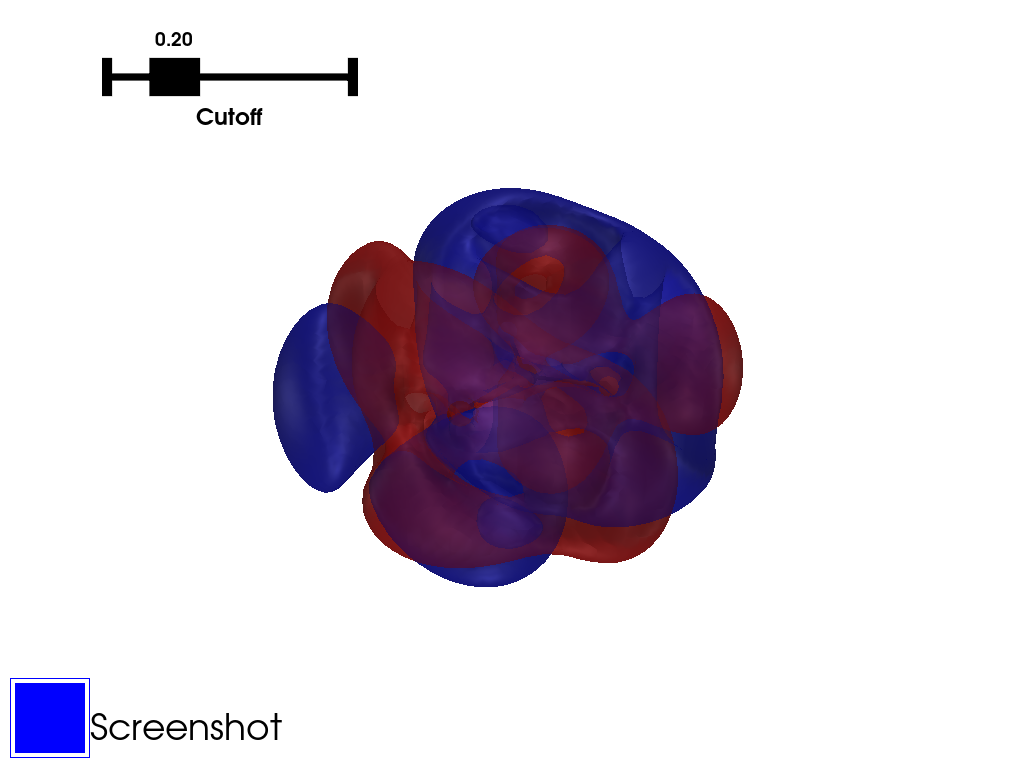
The transition densities can therefore be computed using the MO calculated from molden file combined with the extraction of the coefficients from a TD-DFT calculation.

If one wants to use Orca for the TD-DFT calculation, triplets states should not be included and the keyword TPRINT 0.00001 will allow more transitions to be printed.

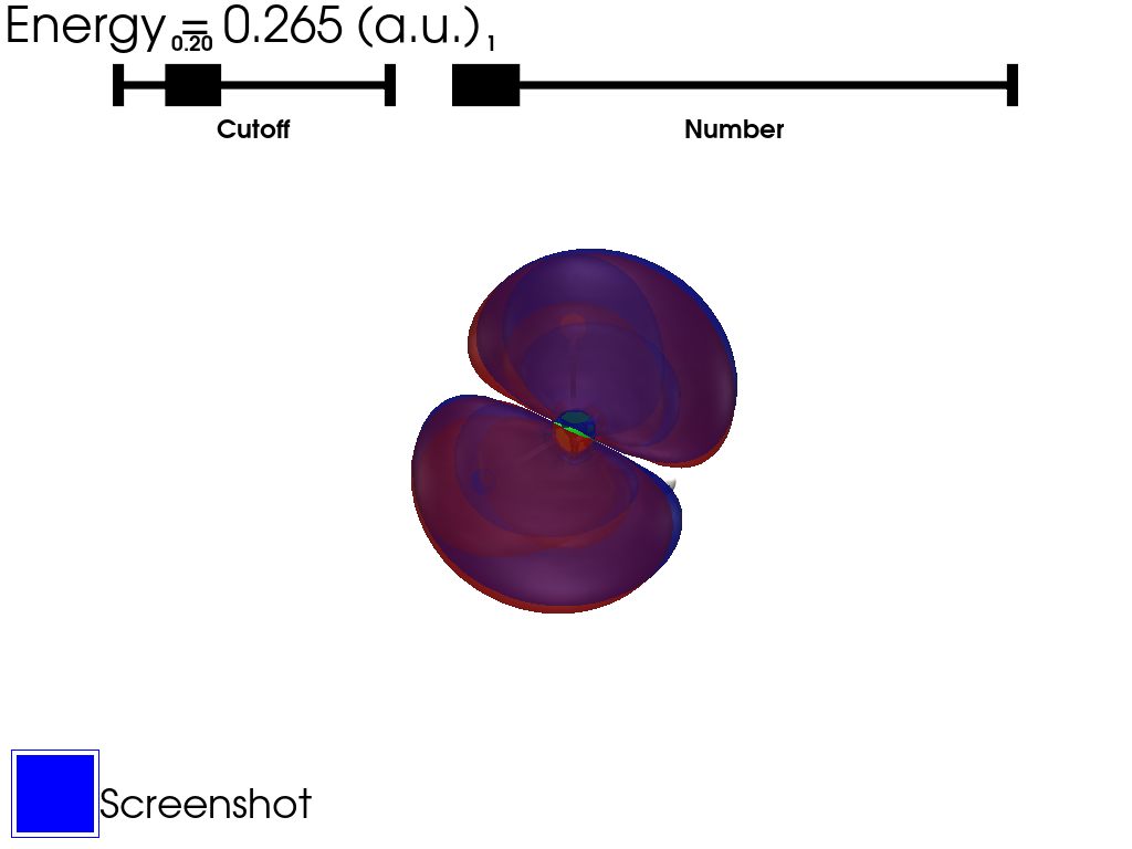
They are sorted by energy. They can be selected using a slider which cannot be accessed using the interactive scene. A script contaning all the examples can be found here.

import rgmol
import rgmol.examples

file = rgmol.examples.molden_CH3Cl
mol = rgmol.extract_molden.extract(file,do_order_bonds=1)
rgmol.extract_orca.extract_properties(rgmol.examples.orca_CH3Cl,mol=mol)
mol.plot_transition_density()
../_images/orbitals-4_00_00.png